tl;dr: Bridson’s algorithm is slow. If you’re considering using it, know that it would be both easier and faster to do dart-throwing with a grid to check validity.
In 2007, Canadian computer scientist Robert Bridson sumbitted a paper to the annual SIGGRAPH conference presenting a new algorithm for generating spacial distributions of points (“Fast Poisson disc sampling in arbitrary dimensions”, available here). Specifically, it’s an algorithm for Poisson disc sampling – generating random, uniformly distributed points with the condition that no two are closer together than some distance Rmin.
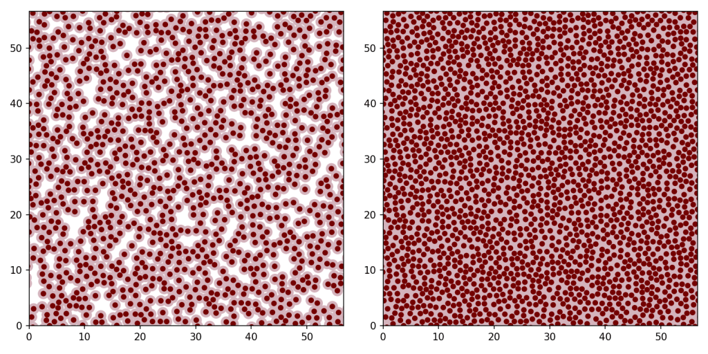
Poisson disc sampling has various applications in image processing, but doing it efficiently is non-trivial. The simplest implementation, sometimes known as dart-throwing, is as follows. Draw a random point uniformly from the domain. Calculate its distance to the nearest previously generated sample. If that distance is less than the minimum distance, discard it. Otherwise, add it to the list of samples. Repeat until you’re happy with the number of points you’ve accumulated, or until the rejection rate gets too high. If you repeat an infinite number of times, you will eventually reach a maximal Poisson disc distribution, with a total point density of around 0.69Rmin−2 (I don’t know why it’s 0.69; I couldn’t find an analytic solution or an explanation in the literature).
The problem with this approach is that to check if a candidate is valid – at least in its most naive implementation – you have to calculate its distance to every previous sample. That makes it a quadratic-time algorithm. In addition, the probability that any given candidate is valid goes to zero as the number of samples increases, meaning that if you want a maximal or nearly maximal distribution, you need to generate and check a huge number of candidates.
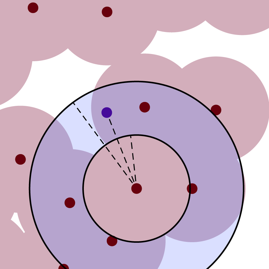
Enter Bridson’s algorithm. Bridson proposed two major changes to the dart-throwing approach to make the process more efficient. First, rather than drawing each candidate randomly from the whole domain, he draws it from an annulus centered on a previous sample, with inner radius Rmin and outer radius 2Rmin. A list is kept of “active” samples from around which candidates can be drawn. Once a certain number of consecutive candidates from a particular annulus are found invalid (Bridson calls this number k and suggests k = 30), that sample is declared infertile and removed from the active list.
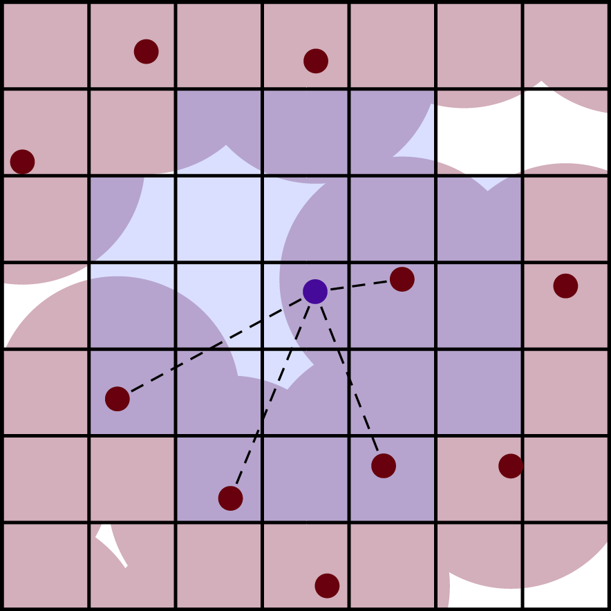
Twoth, he divided the sampling domain into a grid to help with checking the validity of sample candidates. Each grid cell has a reference to all of the samples it contains, if any. This means that, rather than checking the distance to every previous sample, you only need to check the distance to the samples contained in the nearby grid cells. This makes the algorithm linear-time. Bridson scaled his grid so that the cells had diagonals equal to Rmin, ensuring that each contains no more than one sample.
Bridson’s algorithm is the most commonly recommended Poisson disc sampling algorithm on the Internet (see articles by Jason Davies, Manohar Vanga, Hemalatha M., Mike Bostock, and Nicholas Dwork et al.). This is likely due to the grid, which makes Bridson’s algorithm many times faster than the cruder method that preceded it. The annular sampling, however, does not have such a clear benefit. In fact, in addition to making the algorithm more complicated, it actually makes the sampling slightly slower. To demonstrate this, I benchmarked Bridson’s algorithm against two more naive approaches.
First, I implemented a dart-throwing algorithm. Each new candidate is drawn uniformly from the entire domain. Like in Bridson’s algorithm, I use a grid to check each candidate’s validity.
Twoth, I implemented an algorithm that uses the grid cells for sampling. In this one, I keep a list of all empty grid cells and shuffle it into a random order. Each time I want a new candidate, I pop the top cell off of that list and sample a point uniformly from within it. When I run out of cells, I refresh the list and start from the top again. This ensures that I don’t draw candidates from cells that already contain a sample. I also use the grid to check candidates’ validity.
We can easily compare the performance of these two algorithms by plotting the final number of valid samples versus the total number of candidates drawn (normalized to the domain area divided by Rmin2). The number of candidates is proportional to the runtime if we assume that checking the validity of candidates is the slowest step, which my measurements suggest is the case.
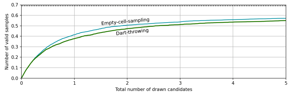
When the first candidates are drawn, almost all of the domain is still valid, so the acceptance rate is nearly 100% and the number of valid samples increases rapidly. As the domain becomes more crowded, though, candidates start to be rejected and the growth rate slows down, eventually asypmtoting to 0.69. As expected, the more complicated empty-cell-sampling method is more efficient than pure dart-throwing; it requires fewer candidates for the same number of valid samples. The difference is pretty modest, though. Since only about one third of the cells actually end up filled in a maximal distribution, excluding them from the sampling domain doesn’t save you all that much time.
What of Bridson’s algorithm? Since it only generates near-maximal distributions, it can’t be plotted in quite the same way. We can still count the total number of candidates generated and compare it to the final number of valid samples, but it’ll be a point instead of a line. That said, we can get multiple points by varying k. Here’s the comparison, zoomed in to the area near the asymptote.
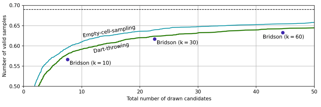
As you can see, Bridson’s algorithm performs similarly to dart-throwing (slightly worse, in fact). This is because Bridson’s method of detecting when an annulus should be marked inactive – by generating a ton of candidates and seeing if any of them are valid – is fundamentally the same as throwing a bunch of darts at the domain and seeing which of them are valid. Reducing k makes this check faster, but results in the algorithm missing more voids and producing a less maximal sample, just like reducing the number of candidates generated when dart-throwing.
I admit I was still surprised to see it perform so poorly, since the annulus system feels like it should efficiently focus on peripheral regions where there are likely to be voids while ruling out areas that have already been covered extensively. However, after thinking about it more, I’ve realized that these annuli are actually an especially inefficient way to partition the domain. Unlike the grid cells that I use to partition the domain in the empty-cell-sampling algorithm, the annuli are heavily overlapping, meaning that you end up having to rule out most parts of the domain multiple times.
It’s worth noting that none of these algorithms are very good if you need really maximal sampling, since near the asymptote, all three generate hundreds of invalid candidates for every valid sample. If you need to make sure your distribution is maximal, and you care about speed, you’ll probably want a more complicated algorithm to more specifically target voids (see, for example, “Efficient maximal Poisson disc sampling” by Mohamed Ebeida et al., available here). But for most people who just want a set of random points that are roughly evenly spaced, dart-throwing is a perfectly serviceable option – you just need to make sure you use a grid to check validity so that it’s linear-time and not quadratic-time.
In conclusion, they have played us for absolute fools, and samples were not supposed to be given annuli. Stop using Bridson’s algorithm!
